Gideon's Wisdom of Crowds Experiment
My grad school friend conducted a fun experiment back in 2012 which I’m embarrassed to say I just learned about. He asked his zillions of Google+ followers to guess the number of cheerios in a jar, hoping to test the idea of the “wisdom of crowds”. He has released the raw data, so I used it as an excuse for another R-tude.
After placing his original spreadsheet into an R dataframe called gideon_woc, I generated this quick overall summary:
gideon_woc %>% group_by(type) %>% summarise(mean = mean(value), median = median(value)) %>% knitr::kable(digits = 0, caption = "Final summary of all data collected.")| type | mean | median |
|---|---|---|
| Combined: All Groups | 514 | 402 |
| GR Group 1 Guesses | 502 | 400 |
| GR Group 2 Guesses | 520 | 420 |
| GR Group 3 Guesses | 525 | 423 |
| GR Group 4 Guesses | 528 | 424 |
| GR Group 5 Guesses | 493 | 400 |
| Shared Group 1 Guesses | 458 | 333 |
| Shared Group 2 Guesses | 485 | 386 |
| Shared Group 3 Guesses | 514 | 348 |
| Shared Group 4 Guesses | 497 | 418 |
| Shared Group 5 Guesses | 221 | 175 |
Gideon received 2,238 valid guesses made in multiple rounds, here organized by type. Some of the people guesses had access to the other people’s guesses (“Shared”) while others were blind to the other guesses (“GR”). Since the actual number of cheerios in the jar is 467, you can see that blinding appears to have made a significant difference in the final guesses.
The good news is that so far our math agrees.
Here’s what we get when we graph each version of the guess. The red dots are outliers, i.e. guesses that fit outside the middle 75% of all guesses.
gideon_woc %>% dplyr::filter(type != "Combined: All Groups") %>% ggplot(aes(x=type,y=value)) + geom_boxplot(outlier.color = "red") + theme(axis.text.x = element_text(angle=90))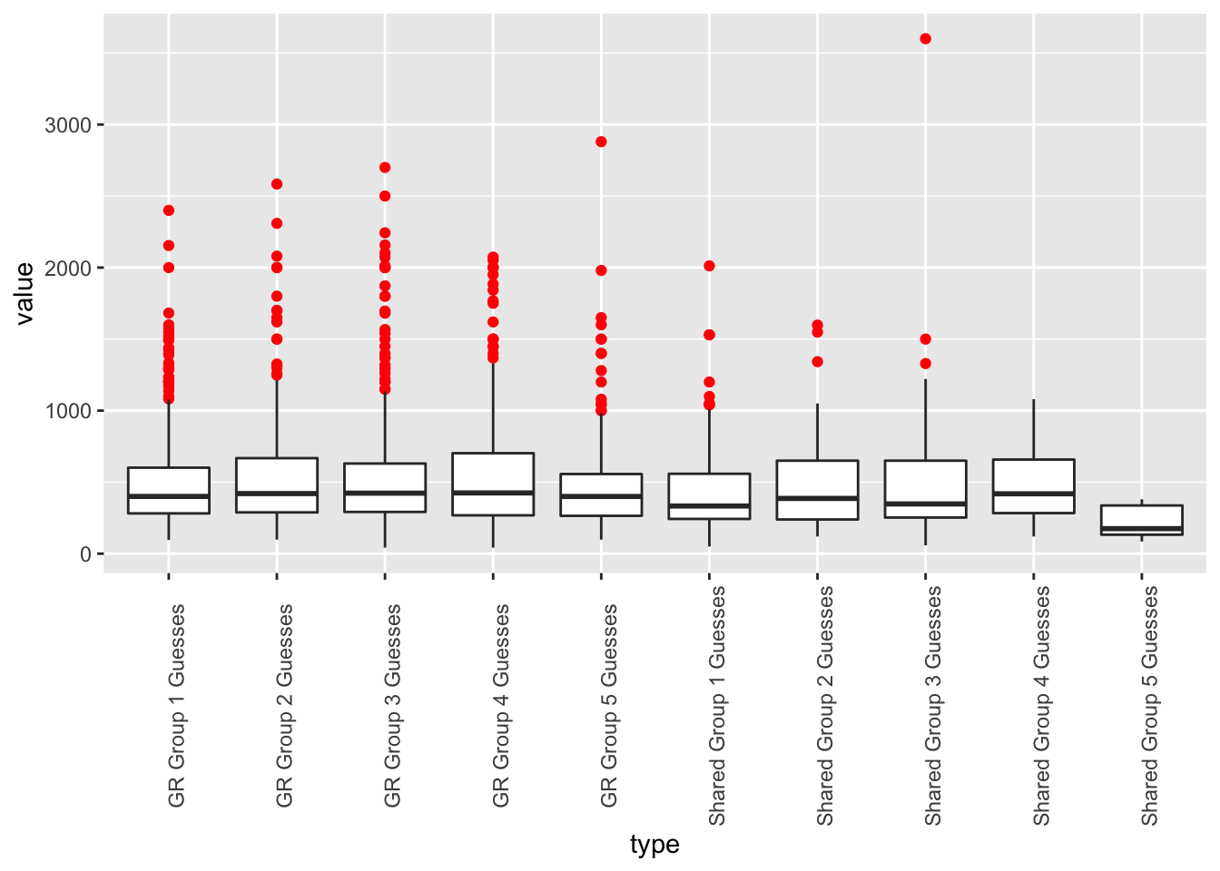
Outliers
One thing that astounds me is the total number of such outliers, as you can see in this table. A lot of people thought the jar contained many multiples more objects than it actually did.
gideon_woc %>%
  group_by(type) %>%
summarise(min = min(value), max = max(value), mean = mean(value), median = median(value)) %>% knitr::kable(caption = "Summary after removing outliers")| type | min | max | mean | median |
|---|---|---|---|---|
| Combined: All Groups | 42 | 3600 | 513.5567 | 402.00 |
| GR Group 1 Guesses | 96 | 2400 | 502.1863 | 400.00 |
| GR Group 2 Guesses | 98 | 2584 | 520.3391 | 420.00 |
| GR Group 3 Guesses | 42 | 2700 | 525.4684 | 423.00 |
| GR Group 4 Guesses | 42 | 2073 | 528.1578 | 424.50 |
| GR Group 5 Guesses | 98 | 2880 | 493.3125 | 399.75 |
| Shared Group 1 Guesses | 50 | 2012 | 457.8618 | 333.00 |
| Shared Group 2 Guesses | 120 | 1598 | 485.4426 | 386.00 |
| Shared Group 3 Guesses | 58 | 3600 | 514.0122 | 347.50 |
| Shared Group 4 Guesses | 120 | 1080 | 497.4000 | 418.50 |
| Shared Group 5 Guesses | 85 | 380 | 220.6667 | 175.00 |
Now let’s remove those outliers and see what we get.
outlier <- function(x) {
  b <- boxplot.stats(x)
  b$out}
outliers <- gideon_woc %>% dplyr::filter(type != "Combined: All Groups") %>% group_by(type) %>% pull(value) %>% outlier()
gideon_woc %>% dplyr::filter(!(value %in% outliers)) %>%
  group_by(type) %>%
summarise(min = min(value), max = max(value), mean = mean(value), median = median(value)) %>% knitr::kable()| type | min | max | mean | median |
|---|---|---|---|---|
| Combined: All Groups | 42 | 1178 | 447.7969 | 390.0 |
| GR Group 1 Guesses | 96 | 1178 | 444.6712 | 396.0 |
| GR Group 2 Guesses | 98 | 1162 | 463.8041 | 400.0 |
| GR Group 3 Guesses | 42 | 1150 | 448.2045 | 400.0 |
| GR Group 4 Guesses | 42 | 1178 | 461.5106 | 401.0 |
| GR Group 5 Guesses | 98 | 1080 | 420.8006 | 374.0 |
| Shared Group 1 Guesses | 50 | 1099 | 396.1875 | 326.5 |
| Shared Group 2 Guesses | 120 | 1050 | 433.1552 | 384.0 |
| Shared Group 3 Guesses | 58 | 1100 | 422.3553 | 325.0 |
| Shared Group 4 Guesses | 120 | 1080 | 497.4000 | 418.5 |
| Shared Group 5 Guesses | 85 | 380 | 220.6667 | 175.0 |
gideon_woc %>% dplyr::filter(!(value %in% outliers)) %>%
  ggplot(aes(x=type,y=value)) + geom_boxplot(outlier.color = "red") + theme(axis.text.x = element_text(angle=90))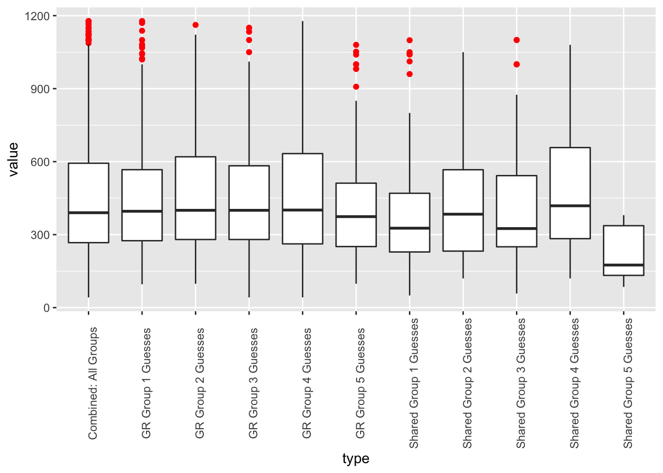
Figure 1: Results after removing outliers
Gideon’s post asks a bunch of questions for statistics experts, hoping to understand just how significant the results were. Unfortunately that’s all the time I have for today. Hopefully I can revisit this post to learn some other interesting insights.