---
title: "What Did McCleary Buy?"
subtitle: "A synthetic-control estimate of Washington's school finance reform"
author: "Richard Sprague"
date: today
---
```{r setup}
#| include: false
source(here::here("R", "00_config.R"))
source(here::here("R", "utils.R"))
source(here::here("R", "04_build_panel.R"))
source(here::here("R", "05_synth.R"))
source(here::here("R", "06_plots.R"))
panel <- build_analysis_panel()
fits <- run_all(panel)
inf <- synth_inference(fits$score)
## Washington 2011 -> 2019 growth as the F-33 pipeline computes it, for the
## comparison against the OSPI figures quoted in "Turning two facts into an estimate".
f33 <- local({
d <- dplyr::filter(panel, state == TREAT_UNIT, year %in% c(2011, 2019))
pc <- function(col) 100 * (d[[col]][2] / d[[col]][1] - 1)
list(
total = pc("rev_pp"),
state = pc("rev_state_pp"),
local = pc("rev_local_pp"),
share_2011 = 100 * d$state_share[1],
share_2019 = 100 * d$state_share[2]
)
})
```
## The question the series asks, and the one it should
The Seattle Times has opened a series, *Educating Washington*, on the perennial
questions of the state's schools. Its first installment asks: *Is WA meeting
its constitutional commitment to education?* [@bazzaz2026paramount]. The
commitment in question is the opening sentence of the constitution's education
article:
> It is the paramount duty of the state to make ample provision for the
> education of all children residing within its borders without distinction or
> preference on account of race, color, caste, or sex.
Dahlia Bazzaz's answer runs mostly through inputs. Since the Supreme Court's
2012 decision in *McCleary v. Washington*, and the $100,000-a-day contempt
fine that followed, K–12 has become the largest item in the state budget. It
bought smaller classes, some of the highest teacher pay in the country, and
per-student spending just above the national average. On that reading, yes:
the state has met its commitment, or at least the court said so when it
released the Legislature from its supervision in 2018.
The series promised a second installment on "what results the state gets, and
doesn't get, for its substantial investment," and that is the better question.
The framers did not write "paramount duty" in order to get a budget line. They
wrote it to get educated children. Whether the state is meeting its commitment
is a question about results, and the constitution's spirit is the standard
that the money is supposed to serve, not the other way around.
The installment has now run [@superville2026spending]. Denisa Superville
reports that state, local, and federal education revenue rose from $13.4
billion in 2012–13 to more than $21 billion in 2024–25, in today's dollars,
while NAEP reading and math scores "inched up then largely flatlined." The
people she interviews then argue past each other. Marguerite Roza of
Georgetown's Edunomics Lab says "we are not seeing any parallel progress in
math and reading given the size of the investments." Superintendent Reykdal
says the results would have been worse without the money. Senate Majority
Leader Jamie Pedersen says there are "too many variables that changed for you
to conclude that our funding was inadequate or a mistake," and calls the
investments "sound."
All three are claims about a counterfactual — what Washington's scores would
have been without McCleary — and none of them is tested against one. The
article does reach for other states: Washington ranks 18th in per-pupil
spending (17th among states; the ranking counts the District of Columbia), 27th of 38 states in math recovery since the pandemic
[@dewey2026recession], and
Mississippi, which spends less, has raised its reading scores. But a ranking
is a snapshot, not a comparison with what Washington itself would have done,
and neither it nor the trend lines shown below can distinguish Roza's reading
from Reykdal's and Pedersen's. This document supplies the missing comparison,
and a benchmark for how large the effect *should* have been.
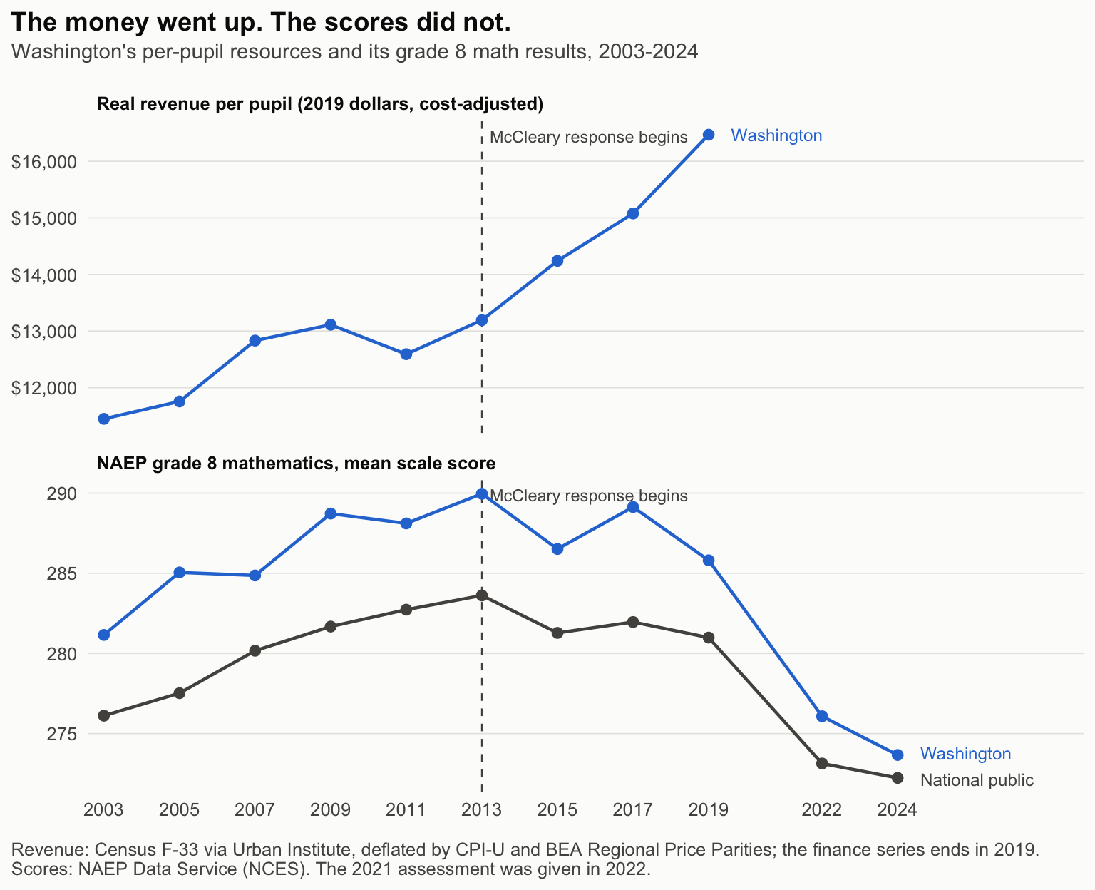
Here is what the results look like, put next to the money, before any
statistical machinery is applied:
```{r}
#| label: fig-money-vs-results
#| fig-cap: "Washington's real per-pupil revenue and its grade 8 math scores, 2003–2024"
#| fig-height: 6.5
naep_all <- build_naep_panel()
wa_pt    <- dplyr::filter(panel, state == TREAT_UNIT)
lead_np  <- naep_all |>
  dplyr::filter(jurisdiction %in% c(TREAT_UNIT, "NP")) |>
  dplyr::select(jurisdiction, year, score) |>
  tidyr::pivot_wider(names_from = jurisdiction, values_from = score) |>
  dplyr::mutate(lead = .data[[TREAT_UNIT]] - NP)
plot_money_vs_results(panel, naep_all)
```
Real, cost-adjusted revenue per student rose
`r sprintf("%.0f%%", 100 * (wa_pt$rev_pp_real[wa_pt$year == 2019] / wa_pt$rev_pp_real[wa_pt$year == 2011] - 1))`
between the last test before the ruling and 2019. Washington's grade 8 math
score, on the one test that is the same in every state, ended that period
`r sprintf("%.1f", wa_pt$score[wa_pt$year == 2011] - wa_pt$score[wa_pt$year == 2019])`
points lower than it began it, and its lead over the national average
slipped from `r sprintf("%.1f", lead_np[lead_np$year == 2011, "lead"])` points
to `r sprintf("%.1f", lead_np[lead_np$year == 2019, "lead"])`. Then came the
pandemic, which took every state down together.
Two lines on a chart are not an estimate. The rest of this document is about
turning them into one: what Washington's scores *would* have been without the
McCleary money, and whether the difference is distinguishable from noise. The
short answer is that it is not. But first it is worth being precise about what
the court actually decided, because a lot of the public argument assumes it
decided something it did not.
## What McCleary actually held
The Supreme Court gets to say what the constitution means, and nothing here
disputes that. But it is worth reading what the court actually said, because
the popular memory of McCleary is that the court found Washington's children
were being shortchanged and ordered the state to fix it. The opinion is
narrower than that, in a way that matters for how the money should be judged.
**The court defined the duty by inputs, not outcomes.** The 2012 opinion
[@McCleary2012] built on a 1978 case, *Seattle School District v. State*
[@SeattleSchoolDistrict1978], which read "ample" to mean "liberal, unrestrained,
without parsimony, fully, sufficient," and read "education" as broad
opportunity: preparing children to "compete adequately in our open political
system, in the labor market, or in the market place of ideas." McCleary
affirmed the trial court's gloss that ample means "considerably more than just
adequate," then stated its own holding in one sentence:
> The "education" required under article IX, section 1 consists of the
> opportunity to obtain the knowledge and skills described in *Seattle School
> District*, ESHB 1209, and the EALRs. It does not reflect a right to a
> guaranteed educational outcome.
The court went further, noting "the inescapable truth that certain factors
critical to a student's achievement are simply outside the State's control."
So to the question of whether McCleary rests on some assumption that every
child starts equal and only money separates them: no. The court expressly
declined to make results the standard. Its holding is about *opportunity*, and
opportunity is measured in what the state provides.
**The finding of underfunding was an accounting finding.** The Legislature had
defined its own "program of basic education." The trial record showed the
state's allocation formulas paid districts less than that program actually
cost: utilities funded at $115 per student against $252 actually spent,
instructional salaries about $8,000 below what districts paid, and so on.
Districts filled the gap with local levies. The court's logic was that "full
funding is whatever the Legislature says it is" amounts to "little more than a
tautology," and that levies, being subject to local votes and local property
wealth, are not the "regular and dependable" revenue the constitution
requires. That is the whole violation: the state was not paying the cost of
the program it had itself defined, and was relying on an impermissible source
to cover the difference.
**Equity enters only through the levy analysis.** The constitution's phrase
"without distinction or preference on account of race, color, caste, or sex"
is recited in the opinion but never applied. The court's equity concern was
between *districts*: property-rich districts can raise more per levy dollar
than property-poor ones. There is no analysis of racial or economic achievement
gaps, and no WASL pass rate or graduation figure anywhere in the part of the
opinion that finds the violation. The achievement statistics that do appear
are quoted from legislative reports as background.
**Compliance was judged the same way.** From the 2014 contempt finding
[@McCleary2014Contempt] through the $100,000-a-day sanction
[@McCleary2015Sanctions] to the order that ended the case
[@McCleary2018Termination], the court "measured progress specifically according
to the areas of basic education identified in ESHB 2261 and the implementation
benchmarks established by SHB 2776": transportation, materials and operating
costs, all-day kindergarten, K–3 class size, and salaries. When it released the
Legislature in June 2018, it did so because the state "has now complied with
this court's orders to fully implement the State's new program of basic
education," while noting in the same paragraph that the plaintiffs "still
dispute the constitutional adequacy of the funding formulas." No outcome
measure appears in any of the seven orders.
So the answer to the Times's question, *is Washington meeting its
constitutional commitment*, has a legal answer and a substantive one. The
legal answer is yes, as of 2018, because the court defined the commitment as
funding a statutory program and the program got funded. The court was candid
that it had done nothing more: it "has not purported to take over public
education" [@McCleary2017Order]. The substantive answer, the one the framers
would have cared about and the one the court explicitly left to the
Legislature and the public, is whether the children are better educated. That
is what the rest of this document tries to measure.
### The results Bazzaz reports
Bazzaz's own survey of outcomes is careful and, on achievement, muted.
Washington performs slightly ahead of the nation in NAEP reading and roughly at
the national average in math, with scores below pre-pandemic levels here as
everywhere. The state's own goal, 90% of students proficient on its state
assessments, sits well above the roughly 70% at grade level in reading and
two-thirds in math. Underneath the averages are sharp disparities: only 42% of
Washington's Latino fourth graders reach NAEP's "basic" level in reading.
State superintendent Chris Reykdal frames the constitutional money as a floor
rather than a program, and puts the open question plainly:
> Money really does matter. But how you deploy it matters too.
That is the question this project takes up, with an explicit counterfactual
rather than a before-and-after comparison. The narrowing matters. This analysis
can say something about grade 8 mathematics, because NAEP provides a comparable
measure across states. It cannot evaluate the two areas where Bazzaz finds
Washington genuinely lagging: preschool access, where the state ranks 7th in
per-child spending but 34th in enrollment, and postsecondary completion, where
its six-year rate of 56.5% is among the nation's worst. Both fall outside the
constitutional guarantee as the court read it, and neither has outcome data
that supports this design.
## What NAEP measures
The **National Assessment of Educational Progress** — "The Nation's Report
Card" — is a federally administered test given to a *representative sample* of
students in every state, not to every student [@naep2024mathematics]. It is run
by the National Center for Education Statistics in grades 4 and 8, in
mathematics and reading, in odd-numbered years (the pandemic pushed the 2021
administration to 2022).
Three properties make it the only usable outcome here:
1. **It is the same test everywhere.** States write their own standards, their
own assessments, and their own definitions of "proficient." Washington's
goal of 90% proficiency is measured on Washington's exam, which tells you
nothing about Oregon. NAEP is a common instrument, which is what makes the
cross-state comparison in this analysis possible at all.
2. **No state can move its own score by redefining the standard.** Because NAEP
is not tied to any state's curriculum or cut scores, it is largely immune to
the standards-inflation that makes state proficiency rates incomparable over
time.
3. **It is reported as a mean scale score**, on a 0–500 scale. This analysis
uses the mean rather than the percent above a proficiency threshold, because
a threshold discards everything about where students sit within a band, and
moves for reasons that have nothing to do with the middle of the
distribution.
The outcome here is **grade 8 mathematics**. Grade 8 has the longest clean
run of state-level results, and mathematics is more responsive to schooling —
and less to home environment — than reading, which makes it the more sensible
place to look for an effect of a school-funding change. Scale scores move
slowly: differences of two or three points between states are small, and the
gap the analysis is trying to detect is of that order.
## Turning two facts into an estimate
Between the 2009–11 and 2019–21 biennia, Washington's state spending on K–12
education rose 110%, while all other state spending rose 52% [@wrc2020mccleary].
Over the same period the state's standing on the National Assessment of
Educational Progress did not improve relative to the rest of the country. In
grade 8 mathematics Washington led the national public average by 5 points in
2003 and by 2 points in 2024.
Those two facts are usually deployed as a rhetorical pair, and the chart
above invites exactly that reading. It should be resisted. Three things have to
be settled before the money and the scores can be compared at all:
1. **How much money actually reached schools per student?** The 110% figure
measures the state budget line. McCleary's central mechanism was a levy
swap — the state assumed obligations previously met by local levies — so
some share of that growth is a change in *who writes the check*, not in how
much is written. Using OSPI's district accounting, the Washington Research
Council reports that from SY 2010–11 to SY 2018–19 total per-pupil revenues
rose 49.7%, state per-pupil revenues rose 81.6%, and local taxes per pupil
fell 0.3% [@wrc2020mccleary].
The pipeline behind this document does not reproduce that last figure. It
uses the Census F-33 survey rather than OSPI's F-196, and over the same
years F-33 puts Washington's local revenue per pupil
**up `r sprintf("%.1f%%", f33$local)`**, with local property tax alone up
14.9% — not flat, and not falling. The two sources agree closely on the
totals (F-33 gives `r sprintf("%+.1f%%", f33$total)` total and
`r sprintf("%+.1f%%", f33$state)` state) and on the direction of the levy
swap: state share of revenue rises about
`r round(f33$share_2019 - f33$share_2011)` points in F-33
(`r sprintf("%.1f%%", f33$share_2011)` to `r sprintf("%.1f%%", f33$share_2019)`)
and about 14 in OSPI (64.6% to 78.4%). They disagree on local revenue in
sign, not just magnitude. The
disagreement is not a definitional one about which local receipts count, and
not a year-alignment artifact; both were checked. It is a genuine difference
between two federal and state collections, and it is left visible here
rather than resolved by picking the more convenient number. Nothing in the
estimates below depends on it: the outcome model uses NAEP scores only, and
the first stage uses total revenue, where the sources agree.
F-33 stops at 2020, but little happens after that. OSPI's
inflation-adjusted total for Washington's K–12 revenue rose from $13.4
billion in 2012–13 to $20.2 billion in 2018–19, then only to $21.0 billion
by 2024–25 [@superville2026spending]. Nearly 90% of the growth had arrived
by the 2019 NAEP administration. Those are totals rather than per-pupil
figures, but the timing is the point: 2019 is when the increase was
complete, not a midpoint. NCES's per-pupil spending series, charted in the
same article, rose 49.1% from 2010–11 to 2018–19, a third source close to
the Research Council's 49.7%.
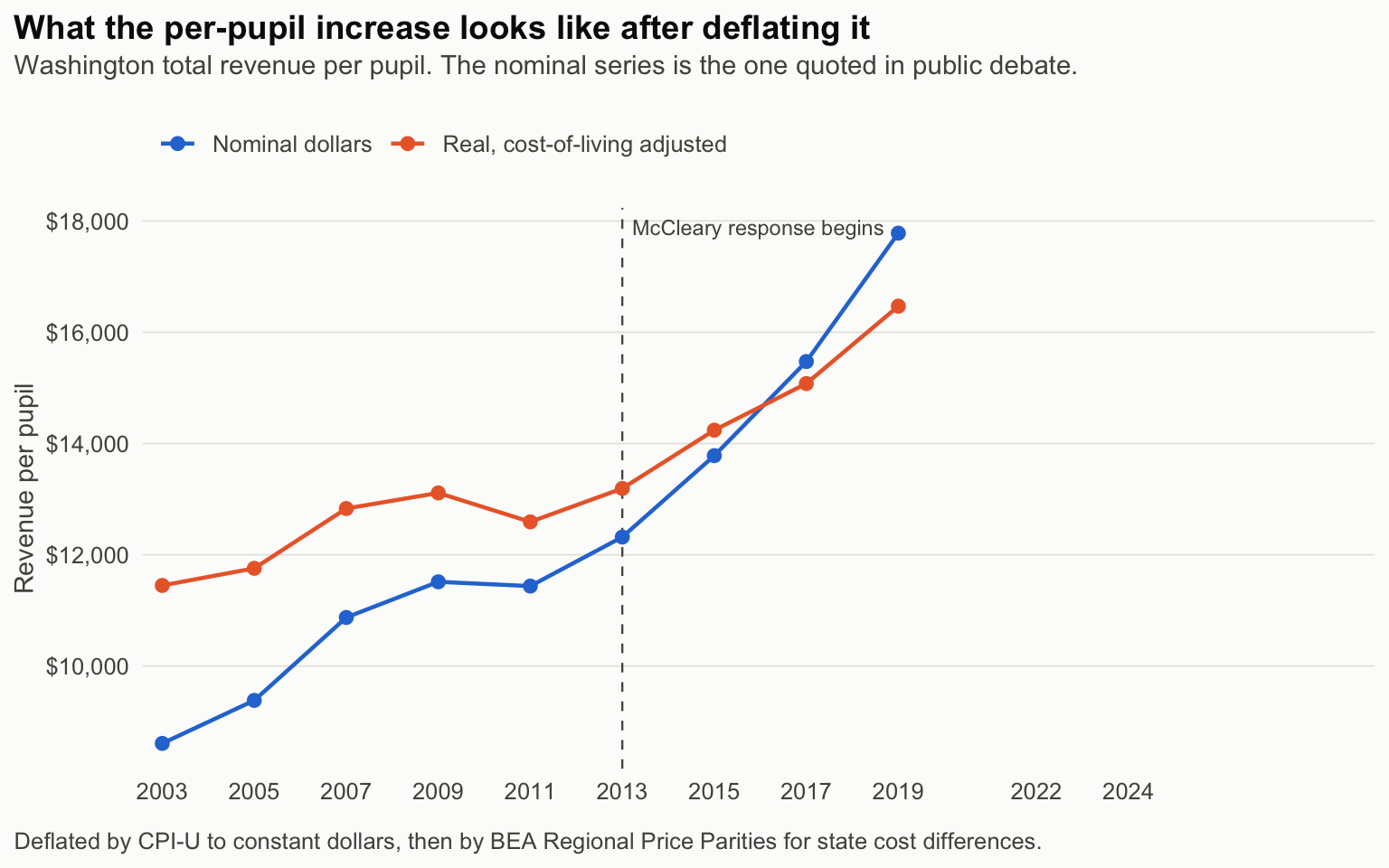
2. **What were those dollars worth?** Nominal per-pupil growth has to be
deflated twice: once for inflation, once for the fact that Puget Sound labor
got more expensive relative to the rest of the country over the same decade.
3. **Compared to what?** Washington's post-2019 scores fell. So did everyone's.
The counterfactual is not "Washington in 2011"; it is "Washington had the
legislature not responded to McCleary."
This project answers the third question with a synthetic control, and carries
the first two through the data pipeline so the resource measure being tested is
one that a skeptic would accept.
## Data
```{r}
#| label: tbl-panel
#| tbl-cap: "Analysis panel coverage"
panel |>
  dplyr::summarise(
    States = dplyr::n_distinct(state),
    `NAEP years` = dplyr::n_distinct(year),
    `First year` = min(year),
    `Last year` = max(year),
    Observations = dplyr::n()
  )
```
Three sources, all public, all pulled by script:
| Source | Series | Access |
|---|---|---|
| NAEP Data Service (NCES) | State mean scale scores, grade 8 math | `R/01_fetch_naep.R` |
| Census F-33 / CCD via Urban Institute | Revenue and expenditure per pupil | `R/02_fetch_finance.R` |
| BEA Regional Price Parities; CPI-U | Place and time deflators | `R/03_price_adjust.R` |
Every API pull is validated against hand-transcribed published figures in
`data/cache/naep_verified_anchors.csv` before the analysis runs
(`make test`). This guards against the failure mode where an upstream schema
change silently returns a different series and the analysis keeps running.
### The spending series, deflated
```{r}
#| label: fig-spending
#| fig-cap: "Washington per-pupil revenue, nominal and deflated"
plot_spending(panel)
```
```{r}
#| label: tbl-spending
#| tbl-cap: "Washington per-pupil revenue by NAEP year"
panel |>
  dplyr::filter(state == TREAT_UNIT) |>
  dplyr::transmute(
    Year = year,
    `Nominal $/pupil` = round(rev_pp),
    `Real, cost-adj. $/pupil` = round(rev_pp_real),
    `State share of revenue` = scales::percent(state_share, accuracy = 0.1)
  )
```
## Design
### One state, no control group
The obvious way to evaluate McCleary is to compare Washington before and after.
That fails immediately, because 2022 and 2024 scores fell across the entire
country. Any before-and-after comparison credits McCleary with a pandemic.
The next idea is to pick a comparison state. But no single state is a good
match for Washington on demographics, economy, and prior test-score trajectory
at once, and whichever one you pick, a skeptic can reasonably accuse you of
having picked it to get the answer you wanted.
**Synthetic control** [@abadie2010synthetic] solves both problems by refusing
to choose. Instead of one comparison state, it builds a weighted average of
many, with the weights chosen by an explicit rule rather than by the analyst.
### What synthetic Washington is
Synthetic Washington is a **weighted average of other states' NAEP scores**,
where the weights are picked so that the weighted average tracks Washington's
actual scores as closely as possible *in the years before 2013*.
Two constraints make it honest:
- **Weights cannot be negative**, so the method can never construct a
counterfactual by subtracting a state.
- **Weights sum to 1**, so synthetic Washington is always an interpolation
among real states, never an extrapolation beyond the range of anything
actually observed.
Concretely, the optimizer in this analysis lands on:
```{r}
#| label: tbl-weights-inline
#| tbl-cap: "The states that make up synthetic Washington"
fits$score |>
  tidysynth::grab_unit_weights() |>
  dplyr::filter(weight > 0.001) |>
  dplyr::arrange(dplyr::desc(weight)) |>
  dplyr::transmute(State = unit, Weight = scales::percent(weight, accuracy = 0.1))
```
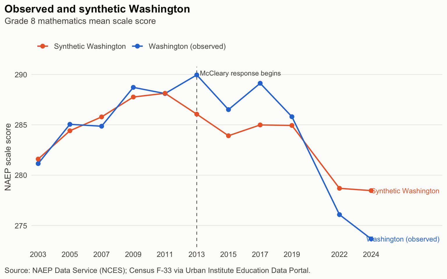
Read that as: the mix of states whose combined grade 8 math path most closely
reproduced Washington's own path from 2003 through 2011. From 2013 onward, that
same fixed mix is carried forward, and **the difference between Washington and
this synthetic Washington is the estimated effect**.
### How the weights are calculated
The weights come from a constrained optimization, not from judgment. The
procedure minimizes the distance between Washington and the weighted donor pool
across a set of **predictors** — here, Washington's NAEP score in each of the
five pre-treatment years (2003, 2005, 2007, 2009, 2011) — subject to the
non-negativity and sum-to-one constraints above. That is a quadratic program,
solved numerically; `tidysynth` hands it to an interior-point solver.
Note what is *not* in the predictor list: per-pupil revenue. Money is the
treatment mechanism, estimated separately below as a first stage, not something
the donor pool is asked to match on. With only five pre-treatment periods, the
predictor set cannot identify more than five predictors — adding spending terms
on top of the five score lags makes the problem numerically singular. `R/05_synth.R`
documents this at the point of decision.
Treatment is dated to **2013**, the first NAEP administration after the January
2012 ruling. The money phased in through 2019, so the estimated effect is a
dose that grows over the post-period rather than a clean step.
The donor pool excludes states with their own major finance-reform shocks in
2008–2022 — `r paste(EXCLUDE_DONORS, collapse = ", ")` — which leaves
`r length(donor_states(panel))` donors. A state that had its own court-ordered
funding overhaul is not an untreated comparison. That exclusion list is the
most contestable input in this analysis; `notes/methodology.qmd` reports how
much it matters, and the short answer is: almost none.
### Placebo tests
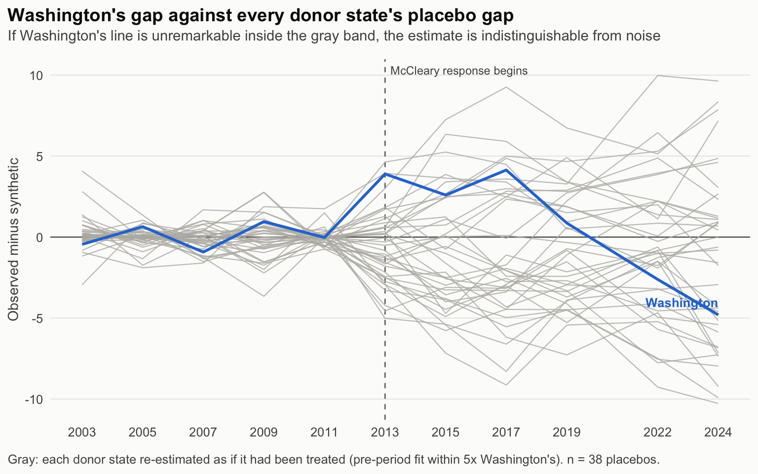
With one treated unit there is no sampling distribution and no standard error
in the usual sense. A gap of four points between Washington and its synthetic
might be an effect, or might be the kind of wobble this method produces
routinely. The only way to know is to find out what "routinely" looks like.
So the procedure is run again, **pretending each donor state was the one
treated in 2013**. Nothing happened to Nebraska in 2013, so whatever gap the
method produces for Nebraska is pure noise — a measure of how much apparent
"effect" this design manufactures when there is nothing to find. Doing this for
every donor gives a distribution of placebo gaps to judge Washington against.
Each unit is scored by its **post/pre RMSPE ratio**. RMSPE is root mean squared
prediction error — the typical size of the gap between a state and its
synthetic. Taking the ratio of the post-treatment value to the pre-treatment
one normalizes for fit quality: a state the donor pool could never match well
to begin with will have large gaps afterward for entirely uninteresting
reasons, and dividing by its pre-period error discounts that.
Rank Washington among those ratios and you get a p-value directly: if
Washington ranks *k*-th of *N*, then *p* = *k* / *N*. It answers the question
"what fraction of states show a post-treatment divergence at least this large
when nothing happened to them?" A Washington that sits unremarkably in the
middle of the placebo pack is a Washington whose gap is indistinguishable from
noise.
## Results
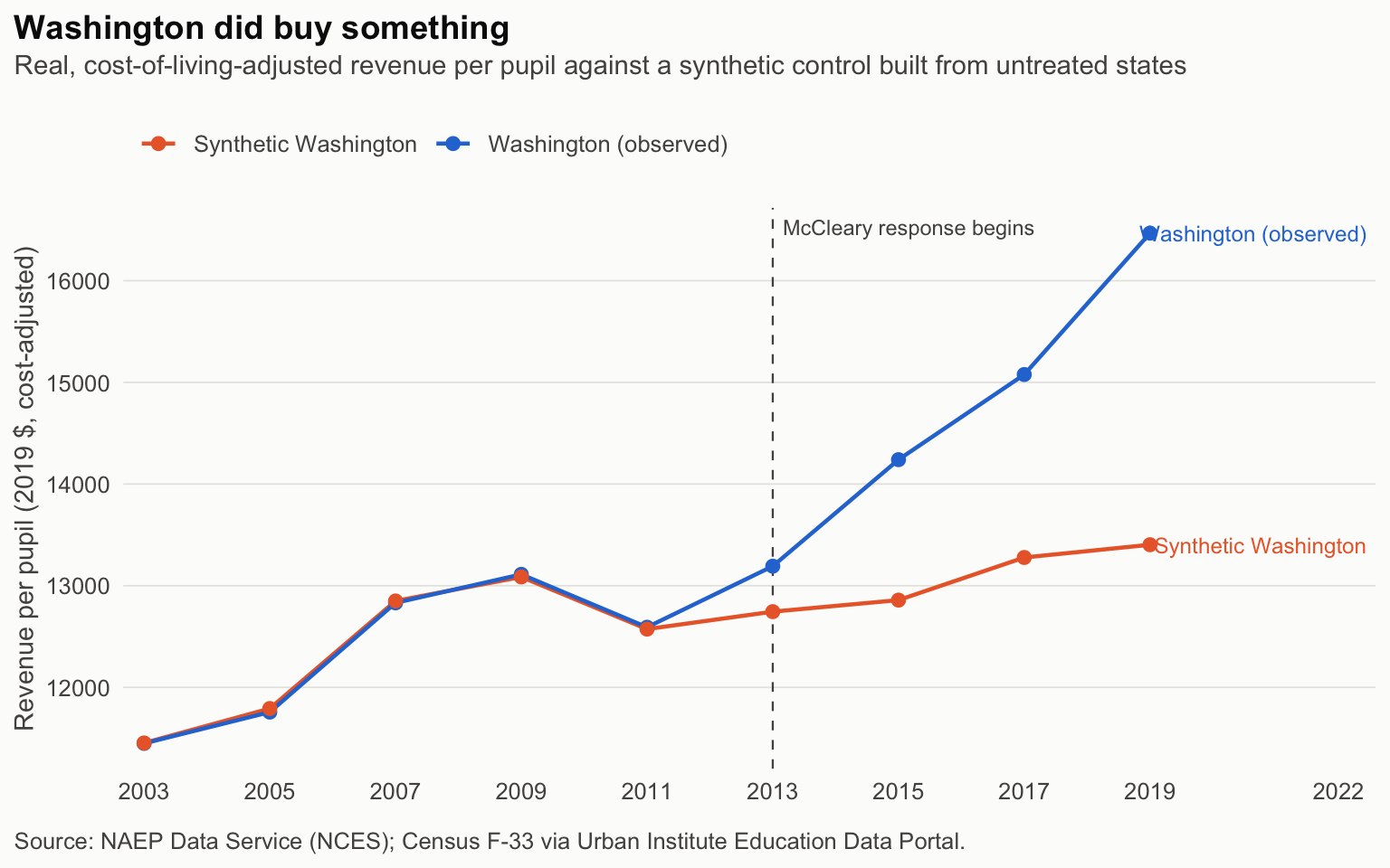
### First stage: did the money actually move?
A finance reform that does not change real resources cannot be tested for
effects on achievement. This is the check that the treatment exists.
```{r}
#| label: fig-first-stage
#| fig-cap: "Real cost-adjusted revenue per pupil: Washington vs synthetic Washington"
plot_trends(
  fits$money,
  title = "Washington did buy something",
  subtitle = "Real, cost-of-living-adjusted revenue per pupil against a synthetic control built from untreated states",
  y_lab = "Revenue per pupil (2019 $, cost-adjusted)"
)
```
### Outcome: NAEP grade 8 mathematics
```{r}
#| label: fig-outcome
#| fig-cap: "NAEP grade 8 math: Washington vs synthetic Washington"
plot_trends(
  fits$score,
  title = "Observed and synthetic Washington",
  subtitle = "Grade 8 mathematics mean scale score"
)
```
```{r}
#| label: fig-gap
#| fig-cap: "Estimated effect: observed minus synthetic"
plot_gap(
  fits$score,
  title = "Estimated effect of the McCleary response on grade 8 math",
  subtitle = "Positive values mean Washington outperformed its synthetic counterfactual"
)
```
### Inference
```{r}
#| label: fig-placebo
#| fig-cap: "Placebo distribution"
plot_placebos(
  fits$score,
  title = "Washington's gap against every donor state's placebo gap",
  subtitle = "If Washington's line is unremarkable inside the gray band, the estimate is indistinguishable from noise"
)
```
```{r}
#| label: tbl-inference
#| tbl-cap: "Post/pre RMSPE ratios, ranked"
inf$table |> head(12)
```
Washington's post/pre RMSPE ratio is `r round(inf$rmspe_ratio, 2)`, ranking
`r inf$rank` of `r nrow(inf$table)` units, giving a placebo-based
*p* = `r round(inf$p_value, 3)`.
## The answer
```{r}
#| label: bound
#| include: false
placebo_gaps <- fits$score |>
tidysynth::grab_synthetic_control(placebo = TRUE) |>
dplyr::mutate(gap = real_y - synth_y) |>
dplyr::filter(time_unit >= TREAT_YEAR, .id != TREAT_UNIT) |>
dplyr::group_by(.id) |>
dplyr::summarise(mean_abs_gap = mean(abs(gap)), .groups = "drop")
wa_abs_gap <- synth_effects(fits$score) |>
dplyr::filter(time_unit >= TREAT_YEAR) |>
dplyr::summarise(m = mean(abs(gap))) |>
dplyr::pull(m)
placebo_median <- stats::median(placebo_gaps$mean_abs_gap)
detect_bound <- stats::quantile(placebo_gaps$mean_abs_gap, 0.95)
money_gap <- synth_effects(fits$money) |>
dplyr::filter(time_unit >= TREAT_YEAR) |>
dplyr::select(time_unit, gap) |>
tibble::deframe()
money_2019 <- money_gap[["2019"]]
## Sensitivity: CPI-U only, no place deflator. The treatment was mostly teacher
## pay, and a wage-sensitive place index partly deflates it away; this bounds
## how much. fit_money(place_adjust = FALSE) in R/05_synth.R.
fit_money_cpi <- fit_money(panel, place_adjust = FALSE)
money_cpi_gap <- synth_effects(fit_money_cpi) |>
dplyr::filter(time_unit >= TREAT_YEAR) |>
dplyr::select(time_unit, gap) |>
tibble::deframe()
money_cpi_rank <- synth_inference(fit_money_cpi)$rank
## Post-treatment score gaps through 2019, as signed strings for the prose.
score_gaps_2019 <- synth_effects(fits$score) |>
dplyr::filter(time_unit >= TREAT_YEAR, time_unit <= 2019) |>
dplyr::pull(gap) |>
sprintf(fmt = "%+.1f") |>
paste(collapse = ", ")
dollars <- function(x) paste0("$", formatC(round(x, -2), format = "d", big.mark = ","))
## Literature benchmark: Jackson & Mackevicius (2024) meta-analysis, 0.0316 SD
## per $1,000 per pupil sustained four years. Student-level SD of NAEP grade 8
## math, national public, from the NAEP Data Service (stattype SD:SD), pulled
## 2026-09-29: 36.42 in 2013, 39.82 in 2019.
JM_SD_PER_1000 <- 0.0316
NAEP_SD <- c(`2013` = 36.42, `2019` = 39.82)
predicted_pts <- money_2019 / 1000 * JM_SD_PER_1000 * NAEP_SD
```
**Did Washington's McCleary response buy measurable achievement? Not
detectably — and the money did arrive, so that is a finding about the
spending, not about missing data. But "not detectable" here includes the
effect the research literature would have predicted, which is a weaker
verdict than "no."**
Two results, and they point in different directions.
**The money is real and large.** By 2019 Washington was spending
**$`r formatC(round(money_2019), format = "d", big.mark = ",")` more per pupil**
than its synthetic counterpart, in inflation- and cost-of-living-adjusted
dollars — a divergence that ranks 4th of 40 units against placebo, with
pre-treatment tracking inside $35. The common objection that McCleary was
merely a levy swap, moving the same dollars from local to state ledgers, does
not survive the correction. Real resources per student rose, substantially,
relative to what would otherwise have happened. Dropping the
cost-of-living adjustment, which partly nets out the teacher raises that made
up most of the treatment, and deflating by CPI-U alone widens the 2019 gap to
$`r formatC(round(money_cpi_gap[["2019"]]), format = "d", big.mark = ",")`, so
the cost-adjusted figure is the conservative one.
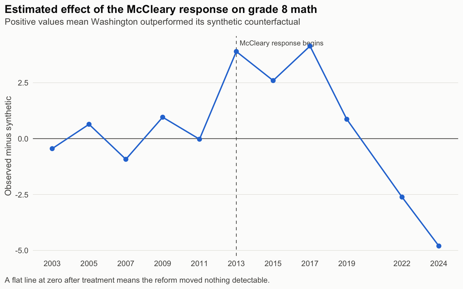
**The achievement gain is absent.** Washington's grade 8 math scores diverge
from synthetic Washington by an average of
**`r round(wa_abs_gap, 2)` scale points** across the post-treatment period. The
median untreated state diverges by `r round(placebo_median, 2)` points, which
is the same number to within a rounding error. Its post/pre RMSPE ratio ranks
`r inf$rank` of `r nrow(inf$table)`
(*p* = `r round(inf$p_value, 3)`), and the result holds whether treatment is
dated 2013, 2015, or 2017, and whether or not the donor exclusions are applied.
### How large an effect could have hidden?
This is the question that separates "no effect" from "no power to see one," and
it deserves a number rather than a caveat.
A sustained divergence would have to average about
**`r round(detect_bound, 1)` scale points** to fall outside the 95th percentile
of what untreated states produce by chance in this design. That is the
detection floor. For scale: Washington's entire lead over the national public
average was 5.0 points in 2003 and 1.4 points in 2024.
The floor only matters next to an expectation, and the school-finance
literature supplies one. Jackson and Mackevicius's meta-analysis of US
spending evaluations finds that $1,000 more per pupil, sustained for four
years, raises test scores by 0.0316 standard deviations on average
[@jackson2024expect]. (It is the same study behind the college-going figure
Superville cites.) Applied to Washington's
$`r formatC(round(money_2019), format = "d", big.mark = ",")` first-stage gap,
and to the student-level spread of NAEP grade 8 math (a standard deviation of
`r sprintf("%.1f", NAEP_SD[["2013"]])` points in 2013,
`r sprintf("%.1f", NAEP_SD[["2019"]])` in 2019), that predicts a gain of
**`r sprintf("%.1f", predicted_pts[["2013"]])`–`r sprintf("%.1f", predicted_pts[["2019"]])`
scale points**.
That is below the detection floor. The effect the literature says McCleary
should have produced is one this design could not have seen. And the
post-treatment gaps actually observed through 2019 (`r score_gaps_2019`)
are about that size. They are indistinguishable from placebo noise, but also
indistinguishable from the benchmark.
The benchmark flatters McCleary in two ways and understates it in one. It
assumes the full increase was in place for four years, but the first-stage
gap was still widening in 2019 (about `r dollars(money_gap[["2015"]])` in 2015 and
`r dollars(money_gap[["2017"]])` in 2017, before the jump to the 2019 figure), so the eighth graders tested that year
had much less exposure than that. It also averages over reforms that
reached poor districts first, and effects are smaller for advantaged students.
McCleary was spread across the whole system. Against that, a statewide mean
understates any gain that went to the students the money was least likely to
reach.
So the honest statement has two halves:
- **An effect large enough to visibly move Washington's standing against the
nation — the kind that would settle the Roza–Reykdal argument — is ruled
out.** Nothing near the detection floor is in the data.
- **The effect the research literature predicts is not ruled out, and could
never have been** with five pre-treatment periods, a biennial test, and a
single treated state. No design built on state-level NAEP means will
resolve it.
Undetectable at this resolution is not the same as zero. Neither side in the
Times article can claim this result: there is no positive effect to point at,
and no evidence that the money underperformed what money usually buys.
::: {.callout-important}
## Three things that constrain the verdict
**The donor pool is concentrated.** Synthetic Washington is
`r scales::percent(max(tidysynth::grab_unit_weights(fits$score)$weight), accuracy = 0.1)`
South Dakota, with 90% of the weight in three states. By the standard set in
`notes/methodology.qmd`, that makes the point estimate illustrative rather than
inferential — the *direction* of the finding is robust across specifications,
but the precise gap in any given year is not.
**2022 and 2024 are pandemic-contaminated.** Both Washington and its synthetic
fall sharply; the negative gaps in those years should not be read as McCleary
failing. Washington's fall likely has an extra cause, which is Pedersen's point.
In January 2021 fewer than 20% of its K–12 students were attending school in
person in any form, one of five states that low, while 15 states were above
90% [@burbio2021splits]. Over the whole 2020–21 year, 58% of Washington
students were in districts with very low access to in-person instruction
[@csdh2022washington]. 2019 is the last clean post-treatment observation, and it is also the
year the money peaked.
**The test's power comes from the placebo distribution, not from theory.** The
5.5-point floor above is an empirical property of this donor pool and this
panel length, not a general statement about synthetic control.
:::
## The students the money was meant to reach
```{r}
#| label: subgroups
#| include: false
source(here::here("R", "07_subgroups.R"))
sub <- run_subgroups(SUBGROUPS[c("hispanic", "nslp")])
sg <- split(sub, sub$label)
pts <- function(x) sprintf("%+.1f", x)
```
Reykdal's own explanation for flat scores is that the money was not enough for
the students who need it most, those in high-poverty communities, and he puts
the remedy at another $1 billion a year. Braun's is that the Learning
Assistance Program, the state's categorical money for struggling students, is
not always used as intended [@superville2026spending]. Both are claims about
*who* the money reached, and a statewide mean can hide exactly that. So the
same synthetic control was rerun on two NAEP subgroup means for grade 8 math:
Hispanic students (23% of Washington's test-takers in 2019, the largest group
after White students) and students eligible for the National School Lunch
Program. Both series are checked against the published 2019 NCES state
snapshots before use.
```{r}
#| label: tbl-subgroups
#| tbl-cap: "Grade 8 math synthetic control by subgroup, 2019. Detection floor and predicted effect as in the statewide analysis above."
sub |>
  dplyr::transmute(
    Group = c(hispanic = "Hispanic", nslp = "Lunch-eligible")[label],
    Donors = n_donors,
    `Revenue gap 2019` = dollars(money_2019),
    `Score gap 2019` = pts(gap_2019),
    `Placebo rank` = paste(rank, "of", n_units),
    `Detection floor` = sprintf("%.1f", detect_floor),
    `Predicted (J&M)` = sprintf("%.1f", jm_pred_2019)
  ) |>
  knitr::kable(align = "lrrrrrr")
```
Neither subgroup diverges. Hispanic students' post-treatment gaps run
`r paste(pts(unlist(sg$hispanic[c("gap_2013", "gap_2015", "gap_2017", "gap_2019")])), collapse = ", ")`
points from 2013 to 2019, ranking `r sg$hispanic$rank` of
`r sg$hispanic$n_units` against placebo (*p* = `r sprintf("%.2f", sg$hispanic$p_value)`).
The 2019 shortfall is the largest in either series, but untreated states
produce gaps that size routinely. Lunch-eligible students track their synthetic
within two points throughout (`r paste(pts(unlist(sg$nslp[c("gap_2013", "gap_2015", "gap_2017", "gap_2019")])), collapse = ", ")`;
rank `r sg$nslp$rank` of `r sg$nslp$n_units`).
This does not rescue either side, for the same reason as before. The detection
floors (`r sprintf("%.1f", sg$hispanic$detect_floor)` and
`r sprintf("%.1f", sg$nslp$detect_floor)` points) again sit above what the
literature predicts (`r sprintf("%.1f", sg$hispanic$jm_pred_2019)` and
`r sprintf("%.1f", sg$nslp$jm_pred_2019)`). Subgroup means are noisier, and the
Hispanic series loses `r length(donor_states(panel)) - sg$hispanic$n_donors` donor states to
suppressed small-sample cells. The prediction is also, if anything, low, since
the meta-analysis finds larger effects for low-income students. Two further
limits apply:
- **The dose is still statewide.** The revenue gap in the table is Washington's
per-pupil increase over the subgroup's synthetic, not dollars that reached
those students. Reykdal's and Braun's claims are precisely that the two
differ, and nothing in state-level finance data can say by how much.
- **"Lunch-eligible" changed meaning at the treatment date.** The Community
Eligibility Provision, available nationally from 2014-15, lets high-poverty
schools serve every student free without individual applications, which
changes who NAEP records as eligible, differently by state. OSPI reports
450,000 more Washington students with free-meal access since 2017
[@superville2026spending]. Treat the lunch-eligible row as the weaker of the
two.
What the subgroup runs do rule out is the strong form of the targeting
argument: that the money produced a large, visible gain for disadvantaged
students which the statewide average concealed. There is none at this
resolution.
## Grade 4 reading, and Mississippi
```{r}
#| label: reading4
#| include: false
r4 <- split(run_reading4(), c("with_ms", "without_ms"))
pct <- function(x) scales::percent(x, accuracy = 0.1)
```
Bellevue's Aramaki points to Mississippi, which spends less than Washington and
has raised its NAEP reading scores [@superville2026spending]. That is a grade 4
reading story, and the analysis above is grade 8 math, so it cannot speak to
it. The same design was rerun on grade 4 reading, the subject and grade where
Mississippi's gains are measured. Mississippi was dropped from the donor pool,
since its reading reforms are a concurrent treatment of their own.
The result is the closest thing to a signal anywhere in this analysis, and it
is still not one. Synthetic Washington tracks the real one tightly before 2013
(pre-period RMSPE `r sprintf("%.2f", r4$without_ms$pre_rmspe)` points), and the
post-treatment gaps through 2019 run
`r paste(pts(unlist(r4$without_ms[c("gap_2013", "gap_2015", "gap_2017", "gap_2019")])), collapse = ", ")`.
Washington ranks `r r4$without_ms$rank` of `r r4$without_ms$n_units` against
placebo (*p* = `r sprintf("%.2f", r4$without_ms$p_value)`), because a good
pre-period fit makes even a modest divergence stand out. But the divergence is
a single 2015 bump that is gone by 2019, the year the money peaked, which is
the opposite of what a funding effect should look like. The detection floor is
`r sprintf("%.1f", r4$without_ms$detect_floor)` points against a literature
prediction of `r sprintf("%.1f", r4$without_ms$jm_pred_2019)`.
Mississippi does not change the comparison either way. It carries
`r pct(r4$with_ms$ms_weight)` of the weight when allowed in the pool (synthetic
Washington's grade 4 reading is mostly
`r state.name[match(r4$with_ms$top_donor, state.abb)]`,
at `r pct(r4$with_ms$top_weight)`), and with it included the rank is
`r r4$with_ms$rank` of `r r4$with_ms$n_units`. Aramaki's point is about
policy, not money: a state that decided every child would read. The same
Stanford–Harvard report that ranks Washington's recovery lists it among ten
states that had adopted fewer than seven of the "science of reading" policy
elements by January 2024. None of the ten improved in reading from 2022 to
2025; Mississippi, with more, did [@dewey2026recession]. Nothing here tests
that. What it shows is that Washington's added money did not buy a
detectable reading gain.
## What this can and cannot settle
**It does** settle the narrow question it was built for: after a large,
court-forced, substantially uniform resource increase, Washington's grade 8
mathematics performance did not diverge from comparable states by any amount
this design can see. The treatment was delivered and the outcome did not move.
**It cannot** tell you whether money works in general. The best-identified
evidence that school spending raises achievement comes from reforms that
targeted low-income districts [@jackson2016effects; @lafortune2018school].
McCleary was substantially uniform, and the accompanying levy cap partly
redistributed *away from* high-levy districts. A null for McCleary is
consistent with progressive finance reform working elsewhere.
**It cannot** evaluate what Bazzaz identifies as Washington's actual weak
spots — preschool access and postsecondary completion
[@bazzaz2026paramount], neither of which the constitutional guarantee covers.
Those need a different design, and the outcome data for them is worse. One
reading of all this is that the paramount-duty clause did exactly what the
court interpreted it to require, funding K–12 to the point where additional
dollars there buy little, while the parts of a child's education with the
weakest measured results are the parts the clause never reached.
Which returns to the question the Times series opened with. Whether Washington
is meeting its constitutional commitment depends on what you take the
commitment to be. If it is the one the court enforced, a funded statutory
program, the state met it in 2018 and the question is closed. If it is the one
the constitution's authors seem to have had in mind, educated children, then
the honest answer from the best comparable measure we have is that the largest
school-funding increase in the state's history has not yet produced evidence
of it — though, on the evidence above, not proof of its absence either. The
second installment of *Educating Washington* reaches the same impasse from
the trend lines alone [@superville2026spending]. Looking at the students the money was
meant to reach, above, does not break the impasse either: state-level subgroup
means carry the same power problem. What could is district-level data, where
the levy cap made the size of the increase vary from one district to the next.
## Reproducing
```bash
make docker-build   # pinned R + Quarto image
make all            # fetch -> test -> render
```
See `notes/methodology.qmd` for specification checks and `README.md` for the
data-refresh cadence.